Intro to Linear Models in R
September 16, 2017
howto notes R study tutorialLinear Models
Much of this carries over from the previous notes on Matrices in R. These notes were compiled while taking Rafael Irizarry’s MOOC on the subject.
\[\mathbf{Y} = \mathbf{\beta} \cdot \mathbf{X} + \mathbf{\epsilon}\]
where each variable represents a vector/matrix:
\[ \mathbf{Y} = \begin{pmatrix} Y_1\\ Y_2\\ \vdots\\ Y_N \end{pmatrix} , \mathbf{X} = \begin{pmatrix} 1&x_{1,1}& \cdots & x_{1,p}\\ 1&x_{2,1}& \cdots & x_{2,p}\\ \vdots\\ 1&x_{N,1}& \cdots & x_{N,p} \end{pmatrix} , \mathbf{\beta} = \begin{pmatrix} \beta_0\\ \beta_1\\ \vdots\\ \beta_p \end{pmatrix} , \epsilon = \begin{pmatrix} \varepsilon_1\\ \varepsilon_2\\ \vdots\\ \varepsilon_N \end{pmatrix} \]
We can simplify the equations, such as Minimizing Residual Sum of Squares, and represent them as a simple equation, where the variables are matrices/vectors.
Minimizing Residual Sum of Squares:
\[(\mathbf{Y}-\mathbf{X}\mathbf{\beta})^\top (\mathbf{Y}-\mathbf{X}\mathbf{\beta})\\ | \\ \text{Take the derivative} \\ \downarrow \\ 2\mathbf{X}^\top(\mathbf{Y} - \mathbf{X} \hat{\beta}) = 0 \\ \downarrow \\ \text{Solve for } \hat{\beta} \\ \mathbf{X}^\top \mathbf{X} \hat{\beta} = \mathbf{X}^\top \mathbf{Y} \\ \hat{\beta} = (\mathbf{X}^\top \mathbf{X})^{-1} \mathbf{X}^\top \mathbf{Y}\]
Calculate the Residual Sum of Squares using matrices in R:
The vector of residuals is given by the difference of \(\mathbf{Y}\) and \(\mathbf{X}\mathbf{\hat{\beta}}\).
\[\text{Residual Sum of Sqaures} = (\mathbf{Y}-\mathbf{X}\mathbf{\beta})^\top (\mathbf{Y}-\mathbf{X}\mathbf{\beta})\]
r <- y - X %*% Beta
# y, X and Beta are matrices


# Old school option to get RSS
rss <- t(r) %*% r

# Faster option
rss <- crossprod(r)
Calculating \(\hat{\beta}\):
# Old school method
betahat <- solve(t(X) %*% X) %*% t(X) %*% y

# Using crossprod()
betahat <- solve(crossprod(X)) %*% crossprod(X,y)

# The easiest method to calculate betahat is using the lm() function though
crossprod(X)is used to calculate \(\mathbf{X}^\top \mathbf{X}\)
tcrossprod(X)is used for \(\mathbf{X} \mathbf{X}^\top\)
When crossprod doesn’t cut it
In certain cases crossprod will not work to give us \(\mathbf{X}^\top \mathbf{X}\) even if the matrix is actually invertible, i.e. has an inverse matrix. For these problems, we’ll use QR decomposition. This is reminiscent of solving simple matrix equations by hand using the techniques described in early lectures from Dr. Gilbert Strang’s Linear Algebra course.
What is QR decomposition?
\[\mathbf{X = QR}\]
where \(\mathbf{Q}\) is a \(N \times p\) matrix such that \(\mathbf{Q^\top Q = I}\) and \(\mathbf{R}\) is a \(p \times p\) upper triangular matrix.
This might be overkill for some, but it helps my understanding to see that actual derivation of the formula. Essentually, we are swapping \(\mathbf{X}\) for \(\mathbf{QR}\) as we solve for the least squares estimate (LSE).
\[ \mathbf{X}^\top \mathbf{X} \boldsymbol{\beta} = \mathbf{X}^\top \mathbf{Y} \\ (\mathbf{QR})^\top (\mathbf{QR}) \boldsymbol{\beta} = (\mathbf{QR})^\top \mathbf{Y} \\ \downarrow \\ \mathbf{R}^\top (\mathbf{Q}^\top \mathbf{Q}) \mathbf{R} \boldsymbol{\beta} = \mathbf{R}^\top \mathbf{Q}^\top \mathbf{Y} \\ \downarrow \\ \text{Recall, } \mathbf{Q^\top Q = I} \ \text{ so we can drop it, and simplify to:} \\ \mathbf{R}^\top \mathbf{R} \boldsymbol{\beta} = \mathbf{R}^\top \mathbf{Q}^\top \mathbf{Y} \\ | \\ \text{Divide both sides by } \mathbf{R}^\top \\ \downarrow \\ \mathbf{R} \boldsymbol{\beta} = \mathbf{Q}^\top \mathbf{Y} \]
QR <- qr(X) # where X is our matrixThe long way – create variables for \(\mathbf{Q}\), \(\mathbf{R}\), and use the backsolve function.
Q <- qr.Q(QR) # use qr.Q to get our Q
R <- qr.R(QR) # use qr.R to get our R

# Use backsolve function to calculate betahat
betahat <- backsolve(R, crossprod(Q,y))
The shortcut – use the solve.qr function.
QR <- qr(X)

betahat <- solve.qr(QR, y)
The lm function

This is what you’ve all been waiting for. You can use the lm or “Linear Model” function to perform a simple regression.
fit <- lm(score ~ player_age + city, data = score_data)

summary(fit)
Linear Models as Matrix Multiplications
A common theme we’re seeing here is simplicity. Again we find that representing these functions as matrix problems helps make things easier to work with.
The sum of squares formula,
\[\displaystyle \sum_{i=1}^{N}(Y_i - \beta_0 - \beta_1x_{i1} - \beta_2x_{i2} - \beta_3x_{i3} - \beta_4x_{i4})^2\]
can easily be written in matrix notation as:
\[(Y - \beta X)^T(Y - \beta X)\]
Linear Model Example
library(RCurl)
library(ggplot2)

url <- getURL("https://raw.githubusercontent.com/genomicsclass/dagdata/master/inst/extdata/femaleMiceWeights.csv")
dat <- read.csv(text = url)

ggplot(dat, aes(x = Diet, y = Bodyweight)) + geom_point(aes(color = dat$Diet))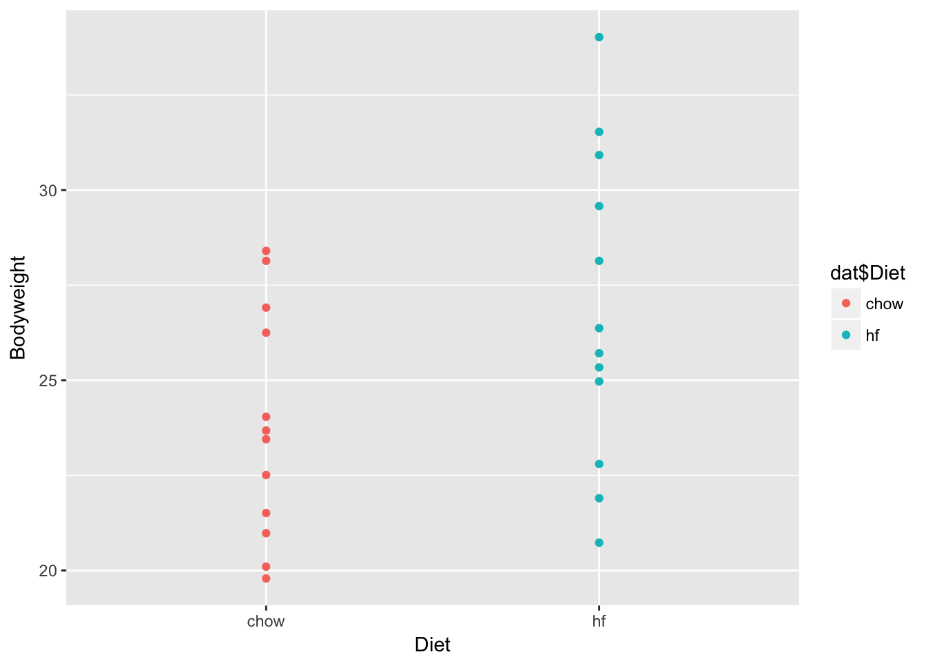
X <- model.matrix(~ Diet, data=dat)
head(X)
## (Intercept) Diethf
## 1 1 0
## 2 1 0
## 3 1 0
## 4 1 0
## 5 1 0
## 6 1 0The indicator variable is the non-reference variable(s). For instance, in the example above with mouse weights, the reference variable is “chow” and the indicator variable is “high-fat.”
levels(dat$Diet)## [1] "chow" "hf"You can change the reference variable using the relevel function.
dat$Diet <- relevel(dat$Diet, ref = "hf")

#flip it back again using relevel
dat$Diet <- relevel(dat$Diet, ref = "chow")
Constructing the linear model
Let’s use the lm function described above to fit our linear model. Our \(y\) variable will be Bodyweight, i.e. modeling bodyweight based on the diet.
fit <- lm(Bodyweight ~ Diet, data = dat)
summary(fit)
##
## Call:
## lm(formula = Bodyweight ~ Diet, data = dat)
##
## Residuals:
## Min 1Q Median 3Q Max
## -6.1042 -2.4358 -0.4138 2.8335 7.1858
##
## Coefficients:
## Estimate Std. Error t value Pr(>|t|)
## (Intercept) 23.813 1.039 22.912 <2e-16 ***
## Diethf 3.021 1.470 2.055 0.0519 .
## ---
## Signif. codes: 0 '***' 0.001 '**' 0.01 '*' 0.05 '.' 0.1 ' ' 1
##
## Residual standard error: 3.6 on 22 degrees of freedom
## Multiple R-squared: 0.1611, Adjusted R-squared: 0.1229
## F-statistic: 4.224 on 1 and 22 DF, p-value: 0.05192The estimate of \(3.021\) as seen in the output tells you the difference between the diet is approximately 3 units of weight. The \(t\) value is merely the estimate divided by the standard error value, i.e. the coefficient value from the first column divided by the error value in the second column.
What exactly is lm() doing? We are fitting our data to a linear model. Essentially it is distilling the math from several lines of code to a few keystrokes. By comparison, below is the lengthier code required to achieve the same result.
y <- dat$Bodyweight
X <- model.matrix(~ Diet, data = dat)
solve(t(X) %*% X) %*% t(X) %*% y
## [,1]
## (Intercept) 23.813333
## Diethf 3.020833The last line is the code version of the following formula to solve for \(\hat{\beta}\).
\[\hat{\beta} = (X^T X)^{-1} X^T y\]
Recall that the above can also be computed using the following formula:
solve(crossprod(X)) %*% crossprod(X,y)where crossprod(X) takes the place of t(X) %*% X and crossprod(X, y) of t(X) %*% y.
Linear Model with 2 variables
url <- getURL("https://raw.githubusercontent.com/genomicsclass/dagdata/master/inst/extdata/spider_wolff_gorb_2013.csv")
spider <- read.csv(text = url, skip = 1)
table(spider$leg, spider$type)
##
## pull push
## L1 34 34
## L2 15 15
## L3 52 52
## L4 40 40X <- model.matrix(~ type + leg, data = spider)
library(rafalib)
imagemat(X, main = "Model matrix for linear model w/ 2 factors")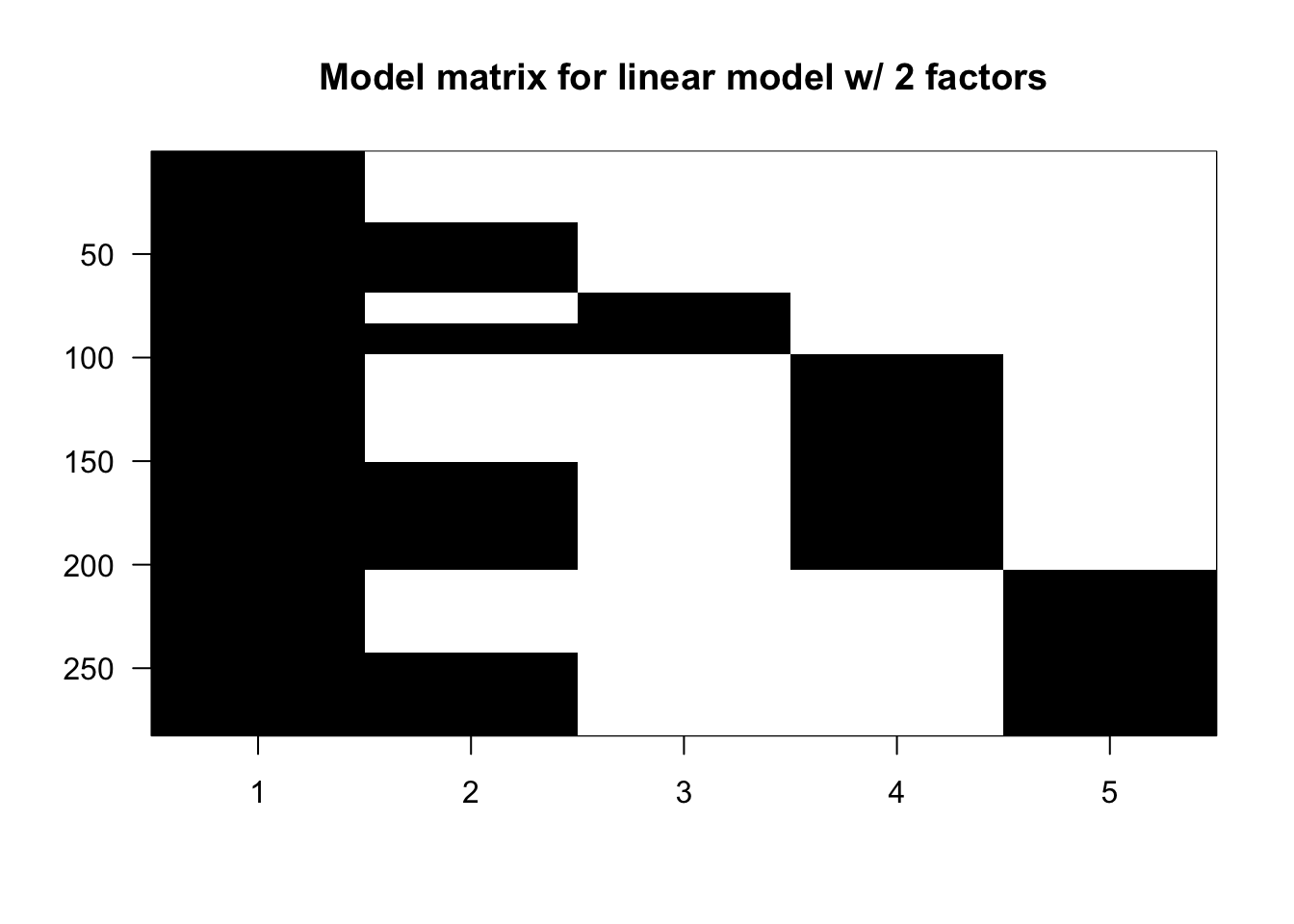
Let’s now fit our model.
fit2 <- lm(friction ~ type + leg, data = spider)
summary(fit2)
##
## Call:
## lm(formula = friction ~ type + leg, data = spider)
##
## Residuals:
## Min 1Q Median 3Q Max
## -0.46392 -0.13441 -0.00525 0.10547 0.69509
##
## Coefficients:
## Estimate Std. Error t value Pr(>|t|)
## (Intercept) 1.05392 0.02816 37.426 < 2e-16 ***
## typepush -0.77901 0.02482 -31.380 < 2e-16 ***
## legL2 0.17192 0.04569 3.763 0.000205 ***
## legL3 0.16049 0.03251 4.937 1.37e-06 ***
## legL4 0.28134 0.03438 8.183 1.01e-14 ***
## ---
## Signif. codes: 0 '***' 0.001 '**' 0.01 '*' 0.05 '.' 0.1 ' ' 1
##
## Residual standard error: 0.2084 on 277 degrees of freedom
## Multiple R-squared: 0.7916, Adjusted R-squared: 0.7886
## F-statistic: 263 on 4 and 277 DF, p-value: < 2.2e-16Linear Models with Contrasts
Appreciate that we have only 5 coefficients, yet are dealing with 8 groups (2 (push/pull) \(\times\) 4 (L1,…, L4)). What is the best we to compare (or should I say contrast) 2 of these groups? You could simply subtract the coefficients to get the difference. However, if you want the standard error and P-value calculations, you will want to use the contrast function from the package of the same name.
Contrast L3 and L2
library(contrast)

L3vsL2 <- contrast(fit2, list(leg = "L3", type = "pull"), list(leg = "L2", type = "pull"))

L3vsL2
## lm model parameter contrast
##
## Contrast S.E. Lower Upper t df Pr(>|t|)
## -0.01142949 0.04319685 -0.0964653 0.07360632 -0.26 277 0.7915Linear Models with Interactions
It’s all about that ‘:’.
X <- model.matrix(~ type + leg + type:leg, data = spider)Now that you understand that, I’ll share with you a cheat code shortcut.
X <- model.matrix(~ type*leg, data = spider)In other words, instead of typing out ~ type + leg + leg:type, you can simply write ~ type*leg.
imagemat(X, main = "Model matrix for linear model w/ 2 factors")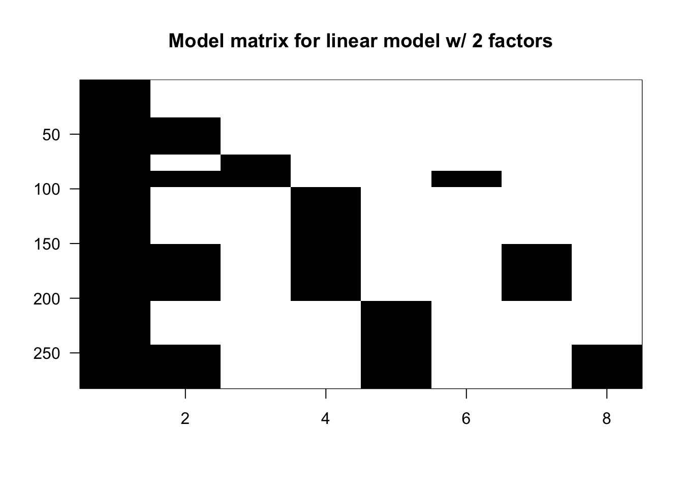
You’ll see that the first 5 columns are the same as we’ve seen before, but now that we’ve introduced the interaction argument, we have 3 new columns at the end.
Fit the Model
fit3 <- lm(friction ~ type*leg, data = spider)
summary(fit3)
##
## Call:
## lm(formula = friction ~ type * leg, data = spider)
##
## Residuals:
## Min 1Q Median 3Q Max
## -0.46385 -0.10735 -0.01111 0.07848 0.76853
##
## Coefficients:
## Estimate Std. Error t value Pr(>|t|)
## (Intercept) 0.92147 0.03266 28.215 < 2e-16 ***
## typepush -0.51412 0.04619 -11.131 < 2e-16 ***
## legL2 0.22386 0.05903 3.792 0.000184 ***
## legL3 0.35238 0.04200 8.390 2.62e-15 ***
## legL4 0.47928 0.04442 10.789 < 2e-16 ***
## typepush:legL2 -0.10388 0.08348 -1.244 0.214409
## typepush:legL3 -0.38377 0.05940 -6.461 4.73e-10 ***
## typepush:legL4 -0.39588 0.06282 -6.302 1.17e-09 ***
## ---
## Signif. codes: 0 '***' 0.001 '**' 0.01 '*' 0.05 '.' 0.1 ' ' 1
##
## Residual standard error: 0.1904 on 274 degrees of freedom
## Multiple R-squared: 0.8279, Adjusted R-squared: 0.8235
## F-statistic: 188.3 on 7 and 274 DF, p-value: < 2.2e-16Contrast the push and pull effect on L2
L2pvp <- contrast(fit3, list(leg = "L2", type = "push"), list(leg = "L2", type = "pull"))
L2pvp
## lm model parameter contrast
##
## Contrast S.E. Lower Upper t df Pr(>|t|)
## -0.618 0.0695372 -0.7548951 -0.4811049 -8.89 274 0C <- L2pvp$X # gives the contrast vector
C## (Intercept) typepush legL2 legL3 legL4 typepush:legL2 typepush:legL3
## 1 0 1 0 0 0 1 0
## typepush:legL4
## 1 0
## attr(,"assign")
## [1] 0 1 2 2 2 3 3 3
## attr(,"contrasts")
## attr(,"contrasts")$type
## [1] "contr.treatment"
##
## attr(,"contrasts")$leg
## [1] "contr.treatment"Difference of differences
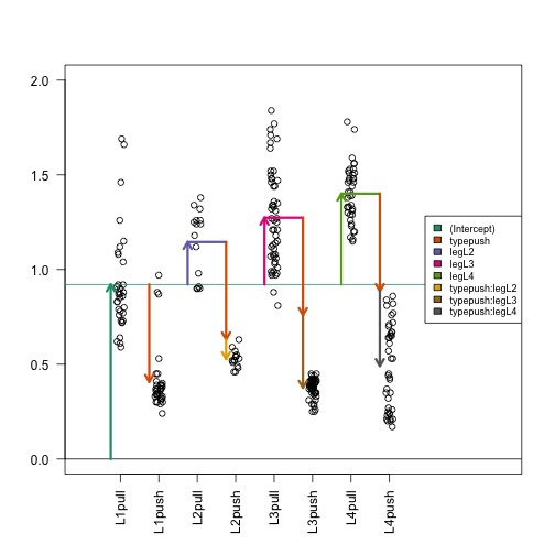
What does “difference of differences” mean? This is best illustrated by an example. I want to compare contrast the push versus pull effect of L3 and that of L2. In the figure below, this is the brown arrow minus the yellow arrow.
Unfortunately, the contrast package won’t work all too well in this instance. We could use some simple math to calculate the difference in the coefficients, but we’re still stuck trying to calculate the standard error, P-value, etc. Fortunately, we can rely on another R package, multcomp.
library(multcomp)
C <- matrix(c(0,0,0,0,0,-1,1,0), 1)
L3vsL2interaction <- glht(fit3, linfct=C)
summary(L3vsL2interaction)
##
## Simultaneous Tests for General Linear Hypotheses
##
## Fit: lm(formula = friction ~ type * leg, data = spider)
##
## Linear Hypotheses:
## Estimate Std. Error t value Pr(>|t|)
## 1 == 0 -0.27988 0.07893 -3.546 0.00046 ***
## ---
## Signif. codes: 0 '***' 0.001 '**' 0.01 '*' 0.05 '.' 0.1 ' ' 1
## (Adjusted p values reported -- single-step method)You’ll notice the following bit of code C <- matrix(c(0,0,0,0,0,-1,1,0), 1) and the use of the linfct = C argument within glht. Essentially, we’re creating a matrix to contrast only those values of interest, which in this case is ‘typepush:legL2’ and ‘typepush:legL3’.
Running coef(fit3) we see that these values are in the 6th and 7th positions.
coefs <- coef(fit3)
coefs
## (Intercept) typepush legL2 legL3 legL4
## 0.9214706 -0.5141176 0.2238627 0.3523756 0.4792794
## typepush:legL2 typepush:legL3 typepush:legL4
## -0.1038824 -0.3837670 -0.3958824Let’s prove that the difference is just the difference between the 6th and 7th coefficients.
coefs[7] - coefs[6]## typepush:legL3
## -0.2798846Notice that this value is the same as what was calculated above using multcomp.
Going back to our example, let us ask the question, “Is the push vs pull difference, different across all the different legs?” So are all of the differences of differences (e.g. the yellow, brown, silver arrows) greater than what we would expect by chance alone?
The t-test allowed us to compute this with head-on comparisons, but now that we are comparing more than 2 groups, we need something a little bit more fancy.
This leads us to the F-test and Analysis of Variance, or ANOVA for short.
anova(fit3)## Analysis of Variance Table
##
## Response: friction
## Df Sum Sq Mean Sq F value Pr(>F)
## type 1 42.783 42.783 1179.713 < 2.2e-16 ***
## leg 3 2.921 0.974 26.847 2.972e-15 ***
## type:leg 3 2.098 0.699 19.282 2.256e-11 ***
## Residuals 274 9.937 0.036
## ---
## Signif. codes: 0 '***' 0.001 '**' 0.01 '*' 0.05 '.' 0.1 ' ' 1Feeling like Noel Gallagher when he goes Champagne ANOVA now.
Collinearity
You can test for collinearity in R using the “Rank” method. The output of this function gives the number of columns that are independent of the others. In a well-designed experiment absent of collinearity, the rank of a matrix (qr(X)$rank) should equal the total number of columns in the matrix (ncol(X)).
# Formula to get the rank of a matrix
qr(X)$rank # where X is the matrix