Probability Distributions in R
September 18, 2017
howto notes R study tutorialProbability Distributions in R
Prefixes:
- p – probability, or cumulative distribution function (cdf), e.g.
pnorm - d – probability density function (pdf), e.g.
dnorm - q – quantile (“inverse” df), e.g.
qnorm - r – random variable of a select distribution, e.g.
rnorm
| Distribution | Core | Parameters | Default Values |
|---|---|---|---|
| Beta | beta |
shape1, shape2 | |
| Binomial | binom |
size, prob | |
| Cauchy | cauchy |
location, scale | 0, 1 |
| Chi-square | chisq |
df | |
| Exponential | exp |
1/mean | 1 |
| F | f |
df1, df2 | |
| Gamma | gamma |
shape, 1/scale | NA, 1 |
| Geometric | geom |
prob | |
| Hypergeometric | hyper |
m, n, k | |
| Log-normal | lnorm |
mean, sd | 0, 1 |
| Logistic | logis |
location, scale | 0, 1 |
| Normal | norm |
mean, sd | 0, 1 |
| Poisson | pois |
lambda | |
| Student | t |
df | |
| Uniform | unif |
min, max | 0, 1 |
| Weibull | weibull |
shape |
Z-score
\[z = \frac{x - \mu}{\sigma}\]
pnorm
Gives the cumulative distribution function (CDF), i.e. the probability that \(X\) will take a value \(\leq x\). It might be easiest to treat \(X\) as your \(z\)-score.
\[F(x) = P(X \leq x)\]
It might be easier to think of the problem as an integration problem.
\[F_X(x) = \displaystyle \int_{-\infty}^x f_X(t)\,\mathrm{d}t\]
pnorm(0) # default mean = 0, sd = 1## [1] 0.5By default, the lower.tail argument is TRUE. If instead, we wished to calculate the probability that \(X\) will take a value \(\geq x\), then we will set lower.tail = FALSE.
pnorm(2, mean = 0, sd = 1)## [1] 0.9772499pnorm(2, lower.tail = FALSE)## [1] 0.02275013Thus, we should expect that the probabilities where lower.tail = TRUE and lower.tail = FALSE shoule equal to \(1\), and we see that is exactly what we get.
pnorm(2) + pnorm(2, lower.tail = FALSE)## [1] 1In a normal distribution that is not skewed, we expect about 50% of the distribution to lie above the mean (and the remaining 50% to be below it). Let’s demonstrate this by generating a sample, e.g. of 200, that follows a normal distribution.
set.seed(1)
X <- rnorm(200) # again, by default mean = 0, sd = 1
hist(X)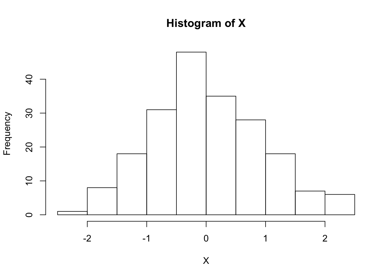
Let’s plot our cumulative distrubtion function (CDF) now.
P <- ecdf(X)
P(0) # should equal ~ 0.5
## [1] 0.53plot(P)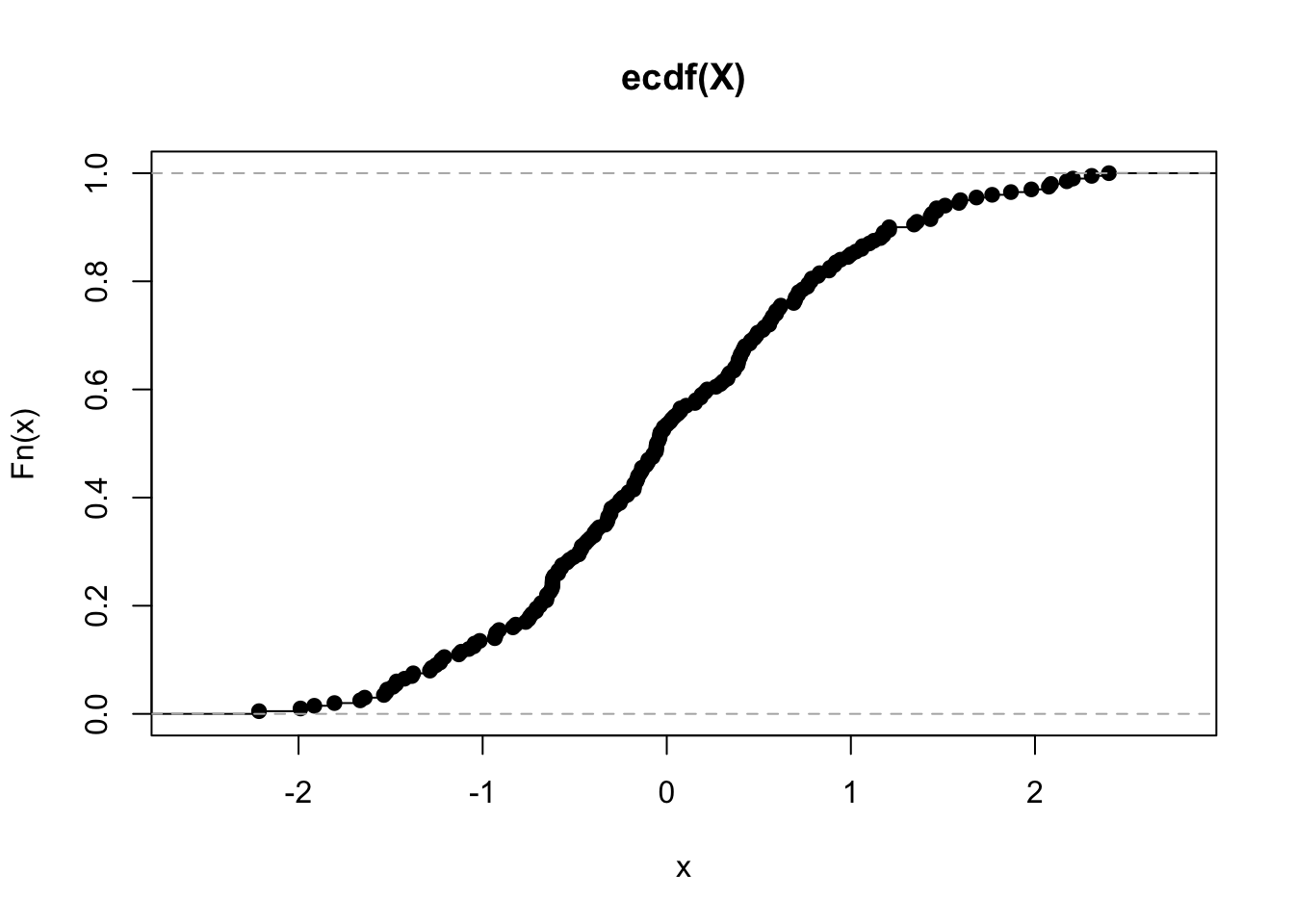
Alternative approach:
x <- seq(-4, 4, by= .1)
y <- pnorm(x)
plot(x,y)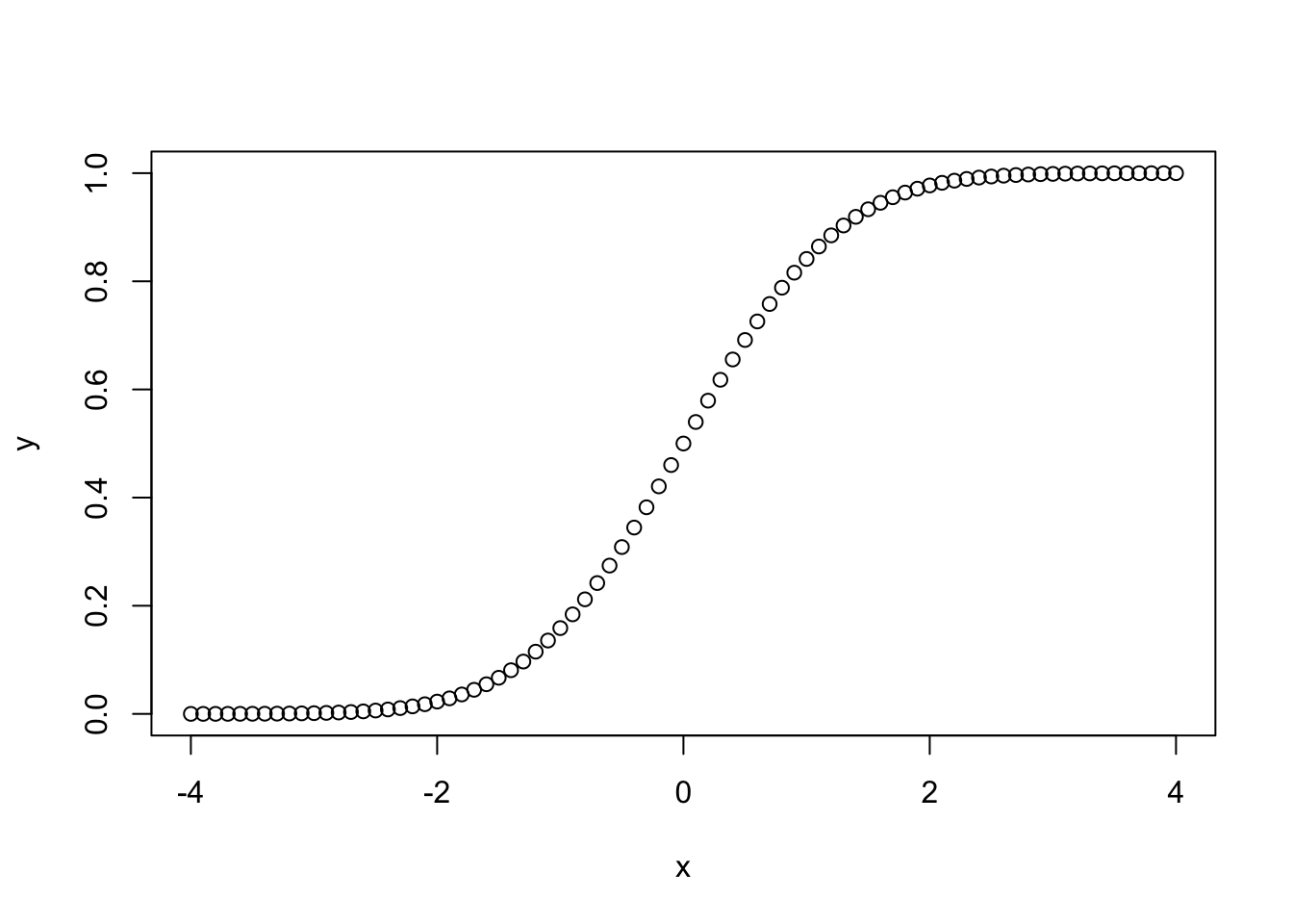
dnorm
The dnorm function gives the height of the probability density function given \(x, \mu,\) and \(\sigma\).
Let’s see the formula of this function to appreciate what the PDF is all about.
\[Pr [a \leq X \leq b] = \displaystyle \int_a^b f_X(x)\,\mathrm{d}x\]
dnorm(0)## [1] 0.3989423The fancier math for a probability density function in a normal distribution is:
\[f(x|\mu,\sigma) = \frac{1}{\sigma\sqrt{2\pi}}e^{-\frac{(x-\mu)^2}{2\sigma^2}}\]
dnorm(0)*sqrt(2*pi)## [1] 1If we solve the equation above, we find that dnorm(0) is equal to \(\frac{1}{\sqrt{2\pi}}\), so multiplying dnorm(0 by \(\sqrt{2\pi}\) gives \(1\) as expected.
Let us now generate a plot of a probability density function (PDF):
z <- seq(-4, 4, by =.1)
y <- dnorm(z)
plot(z, y)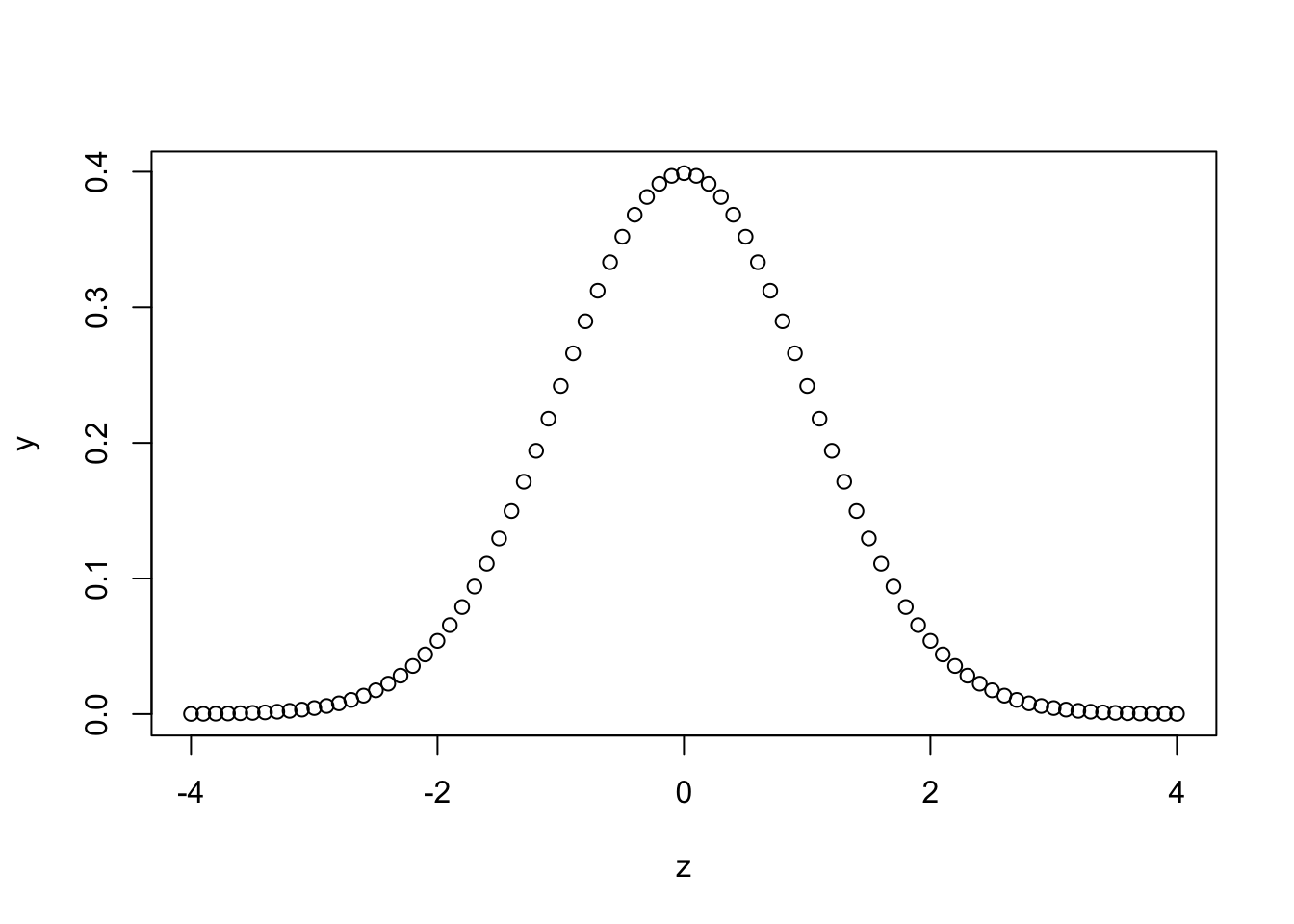
Appreciate that the value of dnorm(0) above corresponds with what is seen in the graph we’ve just plotted for various values. In fact, our series of values, z, can be thought of as \(z\)-scores. Recall, \(z = \frac{x - \mu}{\sigma}\).
qnorm
The thing to know about qnorm is that it is really just the inverse of pnorm. This is best illustrated with some examples. Sean Kross probably said it best, i.e. to think of it as “What is the \(z\)-score of the \(p\)th quantile of the normal distribution?”
pnorm(0)## [1] 0.5qnorm(0.5) ## [1] 0qnorm(pnorm(0))## [1] 0Let’s test it out with some more examples.
# What is the Z-score of the 68th quantile of the normal distribution?
qnorm(0.68)
## [1] 0.4676988# What is the Z-score of the 95th quantile of the normal distribution?
qnorm(0.95)## [1] 1.644854# What is the Z-score of the 99.7th quantile of the normal distribution?
qnorm(0.997)## [1] 2.747781Sources: - Robert and Casella, slide 16 - Sean Kross’s post on the subject