Machine Learning Notes: An Introduction
September 19, 2017
notes study review machinelearningTypes of data
Measurements
- Numerical
- Continuous
- Discrete
- Categorical
- Nominal – unordered
- Ordinal – ordered
- Binary
Types of Variables
- Independent variable, aka predictor or descriptor – variable that does not depend on another, e.g. deomgraphic data such as age, sex, height. This is not under investigator control
- Dependent variable, aka response variable – outcome or output being studied, e.g. clinical outcome or response
- Adjustment variable – counfouder or irrelevant variables that are not being accounted for or studied
- Experimental variable – independent variable under experimenter control, e.g. treatment a patient is randomized to
Notation
- \(n\) – number of distinct data points/observations in the sample
- \(p\) – number of variables available for making predictions
- \(x_{ij}\) – the value of the \(i\)th observation for the \(j\)th variable
- where \(i = 1, 2, \cdots, n\) and \(j = 1, 2, \cdots, p\)
- \(\mathbf{X}\) – a matrix of dimension \(n \times p\), where the \((i, j)\)th element is \(x_{i, j}\)
\[ \mathbf{X} = \begin{pmatrix} x_{1,1}& x_{1,2}& \cdots & x_{1,p}\\ x_{2,1}& x_{2, 2}& \cdots & x_{2,p}\\ \vdots & \vdots & \ddots & \vdots \\ x_{n,1}& x_{n, 2}&\cdots & x_{n,p} \end{pmatrix} \]
- \(y_i\) – the \(i\)th observation of the variable we’re trying to predict
\[ \mathbf{y} = \begin{pmatrix} y_1\\ y_2\\ \vdots\\ y_n \end{pmatrix} \]
Review: Matrix Mutliplication
Example:
\[ \mathbf{A} = \begin{pmatrix} 1&2\\ 3&4\\ \end{pmatrix} , \: \mathbf{B} = \begin{pmatrix} 5&6\\ 7&8\\ \end{pmatrix} \]
A <- matrix(c(1, 2, 3, 4),2,2, byrow = TRUE)
B <- matrix(c(5, 6, 7, 8),2,2, byrow = TRUE)

A %*% B
## [,1] [,2]
## [1,] 19 22
## [2,] 43 50The Basic Formula
In its most simple form, a problem may be expressed as follows:
\[Y = f(X) + \epsilon\]
where \(Y\) represents the response or dependent variable, \(f(X)\) is an unknown function of \(X_1, \cdots, X_p\) inputs (aka features, predictors, independent variable, etc.), and \(\epsilon\) is the error term.
Regression vs Classification Problem
The problem will be considered a regression problem if your output value is a continuous variable. Whereas if your output value is a categorical variable, e.g. Small, Medium, Large or Yes/No, it will be considered a classification problem.
Regression Problem: predict results within a continuous output
Classification Problem: predict results within a discrete output
Estimating \(f\): Prediction and Inference
Prediction
We will attempt to predict \(Y\) using the following basic formula:
\[\hat{Y} = \hat{f}(X)\]
\(\hat{f}\) will not be a perfect estimate for the actual \(f\) because of 2 types of error: reducible and irreducible. Reducible error is minimized by picking the “best” statistical learning technique to estimate \(f\). On the other hand, irreducible error represents the variability in our error term, \(\epsilon\).
Inference
Essentially asking what the relationship is between \(X\) and \(Y\) and how \(Y\) changes as a function of \(X_1, \cdots, X_p\). For example, which predictors (\(X\)) cause the biggest response, is the relationship positive or negative, etc.
Methods: Parametric vs Non-Parametric
Parametric methods rely on a two-step model based approach: 1. Make an assumption about the form/shape of \(f\), e.g. linear 2. Use training data to fit/“train” the specified model
The Parametric method reduces the problem to just determining/estimating a set of parameters (e.g. \(\beta_0, \beta_1,\) etc.), hence the term “Parametric.”
Non-Parametric methods do not makes assumptions about what form \(f\) takes. Rather, these methods try to fit the training data points as best as possible without being too “rough or wiggly.” The downside of Non-Parametric methods is that they require much larger number of observations, \(n\), than do Parametric methods. I believe that Non-Parametric methods are also more prone to the problem of overfitting than its Parametric counterparts.
Model Flexibility Trade-Offs
The Trade-Off b/w Interpretability & Model Accuracy

Generally, less flexible models, such as linear regression and lasso, are more interpretable.
The Bias-Variance Trade-Off
- Variance – the amount by which \(\hat{f}\) would change if we estimated it using a different training data set. In other words, variance is the error from sensitivity to even small fluctuations in the training set, such as \(\hat{f}\) factoring in the noise for its model.
- Example: if a method has high variance, then even small changes in the training data will lead to large changes in \(\hat{f}\).
- Bias – I find this harder to explain, but it’s essentially the inherent error of using a relatively simple model for (complicated) real-life problem. Scott Fortman-Roe puts it this way: “Bias measures how far off in general these models’ predictions are from the correct value.”
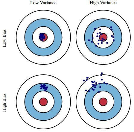
Bias-Variance Trade-Off - similar to explanations of prediction and accuracy in medical school statistics classes. The ideal situation is low variance and low bias.
Generally, \(\uparrow\) model flexibility results in \(\downarrow\) interpretability, \(\uparrow\) variance, and \(\downarrow\) bias.
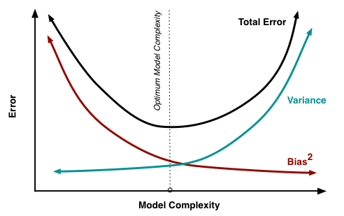
Bias-Variance trade-off against model complexity
Notice that beyond some point (the optimum in the above figure), increasing flexibility has little effect on bias but starts to significantly increase the variance. As this occurs, we start to see the test MSE increase.
Supervised or Unsupervised Learning
Types of Algorithms:
- Supervised Learning
- Unsupervised Learning
- Other:
- Semi-supervised Learning
- Active Learning
- Decision Theory
- Reinforcement Learning
- Recommender systems
Supervised Learning
Definition: working with a labeled dataset, and have some sense that there is some relationship between the input and output.
Often presented as: \({<x_1, y_1>, <x_2, y_2>, ... , <x_n, y_n>}\)
- \(x_n\) are the known data points
- \(y_n\) are the “labels,” e.g. class, value, etc.
Methods:
- Regression Problem: predict results within a continuous output or qualitative variable
- Classification Problem: predict results within a discrete output or quantitative (categorical) variable
Classification

Unsupervised Learning
Definition: working with unlabeled data, i.e. working with \(x_i\) without an associated response variable, \(y_i\).
Data space: \({x_1, x_2, ..., x_n}\)
Methods:
- Clustering
- Density estimation
- Dimensionality reduction
Density estimation:
- Difficult to do in higher dimensions
 Source
Dimenstionality reduction:

alt text
Semi-supervised Learning
Data space: have some \((x, y)\) pairs, but also have some additional \(x_i\) values for which you have no corresponding \(y_1\). Here, we have given/“labeled” points that we can use to predict or impute from our un-labeled \(x\) values.
\[(x_1, y_1), ..., (x_k, y_k), x_{k+1}, ..., x_n\]

Overfitting

The more flexible a training model is, we will often expect to see that the mean squared error (MSE) to decrease.
\[MSE = \frac{1}{n} \displaystyle \sum_{i=1}^{n} (y_i - \hat{f}(x_i))^2\]
Overfitting occurs when our training data generates a small MSE, but our test data gives us a large MSE. Why does this happen? Essentially our algorithm is trying too hard to find patterns in the training data, and in the process may pick up some patterns that are just caused by random chance rather than by true properties of the unknown function \(f\). The Data Skeptic podcast provides a nice intro to overfitting in their mini episode on Cross-Validation.
The training error rate for a classification problem is \[\frac{1}{n} \displaystyle \sum_{i = 1}^{n} I(y_i \neq \hat{y}_i)\]
Generative vs Discriminative Models

As an aside, this image’s font is very Wes Anderson. I like it.
Generative Model
Models the joint distribution, i.e. of \(x\) and \(y\). Often written as \(p(x,y) = f(x|y)p(y)\) or as \(p(x,y) = p(y|x)f(x)\).
Generative model may be limited compared to the discriminative model because you are somewhat confined to working with points within the conditional distribution. For instance, with the image shown above, you may be limited to points within the blue or yellow blobs.
Discriminative Model
Given a set of labeled data, e.g. \({<x_1, y_1>, <x_2, y_2>, ... , <x_n, y_n>}\), and you want to predict its class – \(p(y|x)\).
Bayes Classifier
A simple classification method that assigns each observation to the most likely class, given its predictor values.
\[Pr(Y = j|X = x_0) \: \; \text{where} \, j \: \text{represents the class}\]
For example, if we are dealing with a 2 class model (class 1 or class 2), i.e. 2-dimensional, the Bayes classifier can classify to class 1 if \(Pr(Y=1|X=x_0) > 0.5\) and to class 2 if \(Pr(Y=1|X=x_0) < 0.5\).

k-Nearest Neighbor (kNN)
Given training data \({<x_1, y_1>, <x_2, y_2>, ... , <x_n, y_n>}\), and \(y\) is in some finite space, i.e. \(y \in \{0, 1\}\). If you are now given a new \(x_{new}\), you can use kNN to classify \(y\) for that \(x_{new}\). This is done by taking a “majority vote” of nearby \(x\)’s and their associated \(y\)’s. This is done by computing the distance of \(x_{new}\) from each training point, and then using the sorted distances to select the k nearest neighbors.
For classification, will use “majority rule,” whereas for regression, will use the average value.

Based on the example shown in the image, k = 3 would classify the \(\star\) as Class B by “majority vote.” Setting k = 6, the \(\star\) would then classify as Class A by “majority vote.”